We live in an analogue world, where we can measure height, width, depth, time, luminosity, colour, and sound etc to incredible levels of accuracy until everything smears into a world of utter sub atomic blurriness where nothing seems real any more.

In a digital world all this changes, measurements can now only vary in discrete steps; there are no intermediate values any more! Whether we can tell the difference between our analogue and the digital world is now purely governed by the resolution of our digital measurement scale and the behaviour of our own eyes, ears and brain.

If we decide to measure with a high enough degree of resolution then we find that our eye or ear, or any of our other senses, will accept that the digital representation we have made is an accurate one. If we measure with coarser steps or distort these values then the result can look distinctly unnatural. We will start to notice the dreaded digital artefacts!

But what do digital artefacts look like?

Firstly how many colours do we need to represent the world?

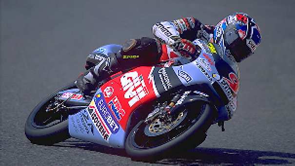
The picture below has been coded to allow up to 16.7 million possible colours (otherwise known as 24-bit colour depth); it looks pretty acceptable as an image.

Let's try reducing the number of colours by reducing the number of bits it takes to represent each picture element.

Now we drop the resolution to only 256 colours, the texture of the track surface has largely disappeared; the surface texture that remains is coarse and funny coloured. The bike has lost its smooth shading too! While undeniably a representation of the original picture, it should fool nobody for long.

Down to just 16 colours now! It makes a stunning graphic, we can see what the picture is, but it's definitely not real.

So that's why mpeg supports 24-bit colour!

Lets try reducing the spatial resolution now, making each pixel twice the size it was originally.

Oh it's gone all lumpy! You can barely read the text on the bike now, - but perhaps if you viewed it from further away it wouldn't look too bad. Try looking at it from 4 times further away!

So the number and size of the pixels we should use to display our pictures is related to the size of the picture we are going to display AND the distance we view it from.

So we have seen all the digital artefacts in this picture then?

Well not quite! Lets take a much closer look, at the top of the rider's helmet and the track immediately behind it.

The track now appears to be made of large greyish rectangular blocks, which seem to pick up shades of pink and blue and green from the helmet, but these colours definitely aren't present on the track!

The helmet itself begins to look like a piece of needlework, with strange rectangular blocks of pixels of the same colour, not showing the gradual colour changes we would expect.

These are definitely digital artefacts too, but where have they come from?

They have come from the image compression technique used for encoding both jpeg still pictures (which was the base coding mechanism used in these pictures) and also mpeg moving pictures: the discrete cosine transform.

How to do the discrete cosine transform.

Here follows an idiots guide to the discrete cosine transform (it has to be an idiots guide; I am, after all, an idiot. Mathematicians please look away - this isn't going to be pretty.)

1. Divide your image into 8x8 pixel blocks.
2. Store the values of each pixel.
3. Calculate the average value of all the pixels in your 8x8 block.
4. Store this average value. This is the first coefficient of your new discrete cosine transform output.
If we only used this first coefficient of the transform for our picture coding we could compress our image by a ratio of 64:1!
The result would be very poor however, as our picture would be made up of very large blocks of these averaged, muddy colours.
(But perhaps this starts to explain where the funny colours on the track behind the motorcyclist's helmet might have come from?)
5. Generate the next coefficients in the transform by dividing the image into four sets of 4x4 pixel blocks, and calculate the average value of each of these blocks. Store the DIFFERENCES between these 4 new 4x4-pixel averages and the original average too. Now we can rebuild our original image with double the accuracy! The result would look less blocky and the colours more realistic.
6. Continue this process - breaking the picture down into 16 sets of 2x2-pixel blocks, then calculating the averages, and storing the differences from the 4x4-pixel averages. Once again we can apply these differences in the reverse direction to get an even more accurate image representation.
7. Then complete the process by taking all 64 pixels 1 at a time and storing the differences between these and the 2x2-pixel blocks. By reversing this process we could get right back to the original image.

But wait a minute, something must be going wrong here!

We started with (8x8)= 64 values, and finished up with (1+4+16+64)= 85 values - what a useless compression scheme this appears to be, we've got more data now, not less!

What we have done is rearranged our input data by storing away the slowest changing picture details first, followed by the slightly faster changing ones, and finally the fastest changing, highest frequency, picture components. But because of the logical way we have performed this transformation we could get back our original picture with 100% accuracy if we wanted to.

Our stored image data is no longer ordered by its spatial position on the screen, but by the range of picture frequencies embedded within the picture.

If we look at 'real world' pictures we notice that the highest frequency picture components usually show very small difference values from the medium frequency components after this transformation. If the differences are near zero it doesn't hurt our visual perception of the picture much if we lose these differences entirely.

So let's throw them away! Its starting to look like we might start to get some compression out of this discrete cosine transform after all.

Let's throw some more data away. Does it really matter if the medium frequency average value differences we have stored are not stored accurately, and we apply some rounding to the figures?

In fact the eye doesn't bother too much about this either, so we can start to do some real compression at last!

Wait a minute, now we've thrown away a lot of the 'invisible' variability from our data, and decided how many of these frequency components we really need to preserve, what would happen if we apply Huffman coding too! We've got ourselves a pretty good compression algorithm!

Its playtime!

Surf off to this site where you will find an interactive demonstration of the discrete cosine transform.

For all you math heads there are some more technical pages there too!

This site lets you draw an 8x8 picture, and apply the discrete cosine transform to it. Not only that, it lets you play with which frequency components are passed through to the final decoded picture.

Start with the simple patterns available on the input buttons, and work your way up to a checkerboard, or any other shape, or try graduated fills, see for yourself which frequency components are important. How much compression can you get away with?

Oh, and one final question. Who is the motorcyclist?

Oh, and one apology. We still don't have any moving pictures, well perhaps next time!

The Professor